2.6 Defining complicated structures

CAMFR has a facility which makes it easier to define complicated non-trivial structures. Rather than manually specifying the geometry slice by slice, we can define a 2D structure in terms of higher level geometric shapes, like circles, triangles or rectangles. This definition can then be automatically discretised and converted to an expression which can be used to initialise a stack.

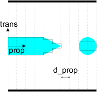
To illustrate this, we model the structure from Fig. 2.5.

#!/usr/bin/env python

####################################################################
#
# Illustrates how to define complicated structures using Geometry.
#
####################################################################

from camfr import *

set_lambda(1)
set_N(40)

air = Material(1)
mat = Material(3)

g = Geometry(air)

g += Rectangle(Point(0.0,-0.5), Point(2.0, 0.5), mat)
g += Triangle (Point(2.0, 0.5), Point(2.0,-0.5), Point(3.0, 0.0), mat)
g += Circle   (Point(4.5, 0.0), 0.5, mat)

set_lower_PML(-0.1)
set_upper_PML(-0.1)

prop0,  prop1,  d_prop  =  0.0, 5.0, 0.50
trans0, trans1, d_trans = -2.5, 2.5, 0.01

exp = g.to_expression(prop0,  prop1,  d_prop,
                      trans0, trans1, d_trans)

s = Stack(exp)

s.calc()

print s.R12(0,0)

The command g = Geometry(air) creates a Geometry object with air as background material. We can subsequently add shapes to this object, e.g. g += Rectangle(Point(0.0,-0.5), Point(2.0, 0.5), mat) adds a rectangle consisting of material mat with given lower left and top right vertices. Note that the first coordinate refers the propagation direction (horizontal in the case of Fig. 2.5).

Other shapes we can add are Circle, Triangle or Square. If two shapes overlap, the shape that was added last takes precedence.

Finally, we can convert the geometry object to an expression which can be used to create a stack. The arguments to this to_expression function are the range and precision in both the propagation and transverse direction (see Fig 2.5).

The increments d_prop and d_trans deserve some additional explanation, because they don't correspond to a uniform rectangular grid. The way the discretisation in performed is as follows. First, the structure is split up into a number of slices in the propagation direction, each d_prop long. Then, subsequent slices are combined if the material discontinuities in the transverse direction are no more than d_trans apart.. This creates some kind of dynamic resolution, because in regions where the shapes vary slower, we will have fewer (but thicker) slices. Also, it makes sure that subsequent identical slices are always combined into one slab. All of this makes for a more efficient discretisation than a traditional uniform grid.

Finally, we want to point out that it's quite easy for the user to add custom shapes by defining a Python object which overloads intersection_at_x. See camfr/geometry.py for more details.

This document was generated by root on August, 27 2008 using texi2html 1.76.