1.6 Example 6: exploiting symmetry

In this example, we will simulate the same structure as in the previous example, but this time we will exploit the symmetry in order to speed up the calculation.

#!/usr/bin/env python

####################################################################
#
# Calculate field profiles in a stack, but exploit symmetry
#
####################################################################

from camfr import *

set_lambda(1)
set_N(10)
set_polarisation(TE)

# Define materials.

GaAs = Material(3.5)
air  = Material(1.0)

# Define stack.

set_upper_PML(-0.1)

set_lower_wall(slab_H_wall)

slab  = Slab(GaAs(.25) + air(2))
space = Slab(air(2.25))

stack = Stack(space(0) + slab(0.5) + space(0))

# Set incident field and calculate stack.

inc = zeros(N())
inc[0] = 1
stack.set_inc_field(inc)

# Save the field to a file.

outfile = file("tutorial6.out",'w')

for x in arange(0.000, 2.250, 0.100):
    for z in arange(0.000, 0.500, 0.010):
        print >> outfile, abs(stack.field(Coord(x,0,z)).E2()),
    print >> outfile

outfile.close()

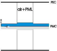
The structure we are studying is symmetric along the horizontal axis. If we want to excite it with a symmetric excitation as well, we can speed up the simulation by introducing a symmetry wall and only calculating half of the structure (fig. 5).

For excitation with the fundamental TE mode, we need to introduce a magnetic wall at the center. This is done with the command set_lower_wall(slab_H_wall) before defining any slabs. lower refers to the bottom side of the slabs (x=0). Obviously, there exists a command set_upper_wall(...) as well. It is also possible to specify a slab_E_wall as boundary condition, but this not necessary as it is the default.

Because the structure now has half the size as the original structure, we can suffice with only half as many modes, which typically buys us a factor eight in computation time.

Another thing to pay attention to is that in this case there is only PML at the upper wall, since the lower wall is effectively the inside of the structure we want to model, so we don't want any absorbing boundary conditions there.

This time, instead of interactively plotting the field, we choose to write it to a file for further analysis. When printing the field, note the trailing command at the end of the print statement. This will prevent the print statement from going to the next line. After we have iterated over all z-values for a given x-value, we force a line break with the command print >> outfile. In this way, the field data is nicely arranged in a matrix format.

This document was generated by root on August, 27 2008 using texi2html 1.76.