| [ < ] | [ > ] | [ << ] | [ Up ] | [ >> ] | [Top] | [Contents] | [Index] | [ ? ] |
The presence of a grating (or a photonic crystal if you prefer), can have a big influence on optical outcoupling. Therefore, CAMFR also contains a library GARCLED for modelling these kinds of grating-assisted resonant-cavity LEDs. The gratings can be placed at the interface between the cavity and the substrate, and/or at the interface between the substrate and the air. Multiple incoherent reflections in the optically thick substrate can also be taken into account.
The following is a simple example:
#!/usr/bin/env python

####################################################################
#
# Extraction efficiency in an organic LED with gratings
#
####################################################################

from GARCLED import *

# Set parameters.

set_lambda(0.565)

orders = 2
set_fourier_orders(orders,orders)

L = 0.400
set_period(L, L)

# Create materials.

Al    = Material(1.031-6.861j)
Alq3  = Material(1.655)
NPD   = Material(1.807)
SiO2  = Material(1.48)
SiN   = Material(1.95)
ITO   = Material(1.806-0.012j)
glass = Material(1.528)
air   = Material(1)

# Define layer structure.

top = Uniform(Alq3,  0.050) + \
      Uniform(Al,    0.150) + \
      Uniform(air,   0.000)

bot = Uniform(Alq3,  0.010) + \
      Uniform(NPD,   0.045) + \
      Uniform(ITO,   0.050) + \
      SquareGrating(L/4, SiO2, SiN, "1", 0.100) + \
      Uniform(glass, 0.000)

sub = Uniform(glass, 0.000) + \
      Uniform(air,   0.000)

ref = Uniform(3) # Don't choose too high: otherwise takes too long

cav = RCLED(top, bot, sub, ref)

# Calculate.

cav.calc(sources=[vertical, horizontal_x], weights=[1, 2],
         steps=30, symmetric=True)

cav.radiation_profile(horizontal_x, steps=30)
|
The main structure of the code should look very similar as compared to the planar case from the previous section.
The command set_period(Lx,Ly) allows you to set the period in the x and y transverse directions. set_fourier_orders(Nx,Ny) sets the number of diffraction orders that are taken into account when simulating the grating with the rigorous coupled wave analysis model (RCWA). This number has a big influence on the calculation time.
Also for reasons of calculation time, the index of the reference material should not be excessively high (but at least as high as the index of the material where the emission takes place).
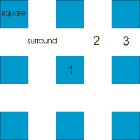
SquareGrating(D, square_m, surround_m, pos, thickness) is a convenience function to create a square grating of squares of material square_m in a background material surround_m. The side of the squares has length D and the period of the grating has already been set by set_period(Lx,Ly). The thickness or height of the grating layer is given by the thickness parameter. The position of the emitting dipole with respect the grating pattern has an influence on the radiation profile. With the pos argument you can specify three different high-symmetry positions '1', '2' and '3'. These are illustrated in the following figure.
For this particular example, the extraction efficiency for the horizontal_x and horizontal_y dipoles will be the same due to symmetry. Therefore, we only calculate the horizontal_x dipole, but give it a weight coefficient of two, so that the average over dipole orientation gives the correct result.
The steps parameter determines in how many equidistant steps the basic integration interval along one k-axis is subdivided. Together with set_fourier_orders(Nx,Ny), these are the main parameters that determine accuracy and calculation time.
symmetric=True tells the software that the grating together with the dipole orientation possess mirror symmetry along the x and y axis. This allows the integration to be restricted to positive values of kx and ky, resulting in a factor 4 speedup.
cav.calc() also returns an object containing all the results, which can be queried in exactly the same way as for the planar case.
Finally, cav.radiation_profile(horizontal_x, steps=30) calculates the TE and TM polarised radiation profile for a single source orientation. This functions in exactly the same way as in the planar case, e.g. it also supports the same optional arguments: radiation_profile(source, steps=30, location='out', density='per_solid_angle', show=True, filename=None). The return values of this function are similarly k, P_TE, P_TM, where k is a 1D vector containing the k-values which are used both for kx and ky. P_TE and P_TM are matrices.
There is also a function to create a square grating with round holes: SquareGratingRoundHoles(D, dx, dy, core_m, surround_m, pos, thickness). Here, dx and dy are the same discretisation parameters used for Geometry (See section Defining complicated structures).
To show how you can manually create different unit cells which are not covered by the convenience functions, we will now explain the code behind the SquareGrating at position 1. As shown in the following figure, the unit cell is built up from three vertical slices, which are represented in the following code by the Slabs s1, s2 and s1. These are then combined in a BlochSection.
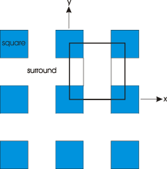
s1 = Slab(square_m(D/2.) + surround_m(_Ly-D) + square_m(D/2.)) s2 = Slab(surround_m(_Ly)) grating = BlochSection(s1(D/2.) + s2(_Lx-D) + s1(D/2.)) |
To use this grating object in your stack definition, just do the following:
bot = Uniform(Alq3,  0.010) + \
      Uniform(NPD,   0.045) + \
      Uniform(ITO,   0.050) + \
      grating(0.010) + \
      Uniform(glass, 0.000)
|
In reality, the dipole position will be random with respect to the grating. The following code illustrates a more elaborate example, where the emission is averaged over the three high-symmetry dipole positions. Also, the structure is calculated for several grating parameters.
#!/usr/bin/env python

######################################################################
#
# Extraction efficiency in an organic LED with gratings
# averaged over dipole position.
#
######################################################################

from GARCLED import *

def calc(L, h, D, orders, wavelength=0.565):

  # Set parameters.

  set_period(L, L)

  set_lambda(wavelength)

  set_fourier_orders(orders, orders)

  print
  print "wavelength, orders L h:", wavelength, orders, L, h

  # Create materials.

  Al    = Material(1.031-6.861j)
  Alq3  = Material(1.655)
  NPD   = Material(1.807)
  ITO   = Material(1.806-0.012j)
  SiO2  = Material(1.48)
  SiN   = Material(1.95)
  glass = Material(1.528)
  air   = Material(1)

  eta_sub, eta_out = [], []

  # Define layer structure.

  for pos in ['1', '2', '3']:

    print
    print "*** Position", pos, "***"
    print

    top = Uniform(Alq3,  0.050) + \
          Uniform(Al,    0.150) + \
          Uniform(air,   0.000)

    bot = Uniform(Alq3,  0.010) + \
          Uniform(NPD,   0.045) + \
          Uniform(ITO,   0.050) + \
          SquareGrating(D, SiO2, SiN, pos, h) + \
          Uniform(glass, 0.000)

    sub = Uniform(glass, 0.000) + \
          Uniform(air,   0.000)

    ref = Uniform(3) # Don't choose too high: otherwise takes too long

    cav = RCLED(top, bot, sub, ref)

    # Calculate average over source orientation for a given position.

    res = cav.calc(sources = [vertical, horizontal_x, horizontal_y],
                   steps=100, symmetric=True)

    eta_sub.append(res.eta_sub)
    eta_out.append(res.eta_out)

    sys.stdout.flush()

    free_tmps()

  # Print average over position and source.

  print
  print "*** Averaged over dipole position and source orientation ***"
  print
  print "Averaged extraction efficiency to substrate            :", \
                                                        average(eta_sub)
  print "Averaged extraction efficiency to bottom outside world :", \
                                                        average(eta_out)

# Loop over period and thickness of the grating.

for L in [.300, .500, .700]:
  for h in [.100, .200, .400]:
    calc(L, h, L/2, orders=3)
|
A grating close to the light emitting layer will have an influence on the extraction of the light trapped inside the active layers. However, as the figure below illustrates, this grating can also help to couple out light trapped inside the substrate, provided the lateral extent of the device is sufficienly large.
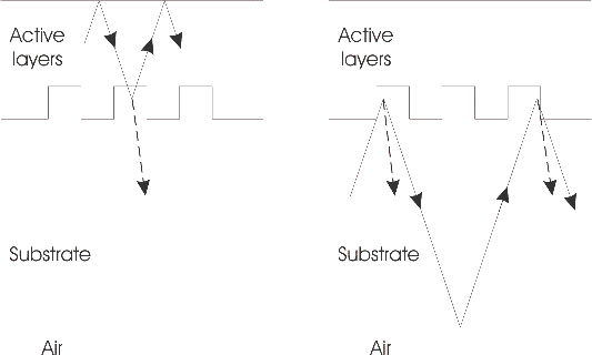
These multipass effects in the substrate happen incoherently because of the large thickness of the substrate. Normally, they are not taken into account, i.e. the substrate is considered to be single-pass. You can calculate the multipass effects by specifying the optional parameter single_pass_substrate=False to cav.calc().
Finally, instead of placing the grating at the cavity-substrate interface, you can place it at the substrate-air interface by including a grating in the sub stack. In this case, the grating will only have an influence on the substrate modes, and you need to specify single_pass_substrate=False.
| [ < ] | [ > ] | [ << ] | [ Up ] | [ >> ] |
This document was generated by root on August, 27 2008 using texi2html 1.76.