1.1 Example 1: a simple waveguide example

The examples in this chapter can be found in the directory examples/tutorial in the main CAMFR directory. If you're on a Windows system, this directory could by something like C:\python23\Lib\site-packages\camfr, on a Unix system it is usually /usr/lib/python2.5/site-packages/camfr.

The first file tutorial1.py introduces some simple waveguide simulations and looks like this:

#!/usr/bin/env python

####################################################################
#
# Simple waveguide example
#
####################################################################

from camfr import *

set_lambda(1)
set_N(20)
set_polarisation(TE)

# Define materials.

GaAs = Material(3.5)
air  = Material(1.0)

# Define waveguide.

slab = Slab(air(2) + GaAs(0.5) + air(2))

slab.calc()

# Print out some waveguide characteristics. 

print slab.mode(0).kz()
print slab.mode(1).n_eff()
print slab.mode(2).field(Coord(2.25, 0, 0))
print slab.mode(3).field(Coord(2.25, 0, 0)).E2()
print slab.mode(4).field(Coord(2.25, 0, 0)).E2().real


# Do some interactive plotting.

slab.plot()

The first line #!/usr/bin/env python is an optional Unix incantation to tell the operating system that it should execute this script with the Python interpreter.

The next lines illustrate that comments in Python start with #.

The line from camfr import * informs Python that we want to start using the CAMFR library.

The following lines are pretty self-explanatory:

set_lambda(1)
set_N(20)
set_polarisation(TE)

We set the wavelength to 1 micron, use 20 eigenmodes to expand the field, and deal with TE polarisation. Next, we define GaAs to be a material with refractive index 3.5 and air as a material with index 1:

GaAs = Material(3.5)
air  = Material(1.0)

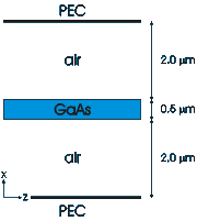
We can now define a simple slab waveguide, with a GaAs core of half a micron thick, and air cladding layers of 2 micron thick.

slab = Slab(air(2) + GaAs(0.5) + air(2))

This structure is implicitly assumed to be sandwiched between two perfect electric conductors (PECs), as indicated in fig. 1:

This figure also indicates the conventions for the coordinate system. The x-axis lies along the cross-section of the slab waveguide and starts at the bottom wall. The waveguide is uniform in the y- and z- direction. The eigenmodes of the waveguide propagates along the z-direction.

Using the command slab.calc(), CAMFR will calculate the properties of the slab, some of which are then printed out in the following lines of the Python script.

print slab.mode(0).kz() prints out the propagation factor of the fundamental mode of the slab, while slab.mode(1).n_eff() displays the effective index of the first order mode.

print slab.mode(2).field(Coord(2.25, 0, 0)) shows the field of the second order mode at x=2.25, which is in the center of the core. This field consists of six complex numbers. E1, E2, Ez are the phasors for the components of the electric field, and H1, H2, Hz represent the magnetic field. Here, 1 refers to the x-direction and 2 to the y-direction. (For cylindrical structures, 1 refers to the radial direction and 2 to the angular direction.)

print slab.mode(4).field(Coord(2.25, 0, 0)).E2().real illustrates how we can extract the real part from a complex number in Python. (real is a built-in Python attribute of a complex number, and as such requires no extra parentheses.) Similarly, the imaginary component can be extracted with imag.

Finally, slab.plot() shows a widget which can be used to interactively explore the properties of the waveguide modes, field profiles and effective index distribution. Note that you can zoom in these plots by drawing a rectangle with the left mouse button pressed. You can also bring up the effective index distribution in the complex plane and click on the modes in that plane to plot their field profiles.

The Python script can be executed in a number of ways. You can type python tutorial1.py, or under Unix you can just suffice by typing tutorial1.py, provided the first line of your script contains #!/usr/bin/env python and the script file's executable bit is set (with chmod +x tutorial1.py). (Note: all of these command need to be typed in on the system prompt, not on the Python prompt.)

Regardless of the invocation method, the output that will be printed out will look something like this:

CAMFR 1.3 - Copyright (C) 1998-2007 Peter Bienstman - Ghent University.

(21.3499038707+0j)
(3.07668661368+0j)
E1=(0,0), E2=(-16.0633,0), Ez=(0,0)
H1=(0.105632,0), H2=(0,0), Hz=(0,0.0966439)
(24.2902148016+0j)
0.649002451002

There is also a third way of starting the script, which is python -i tutorial1.py. This will print out the same output, but will afterwards present you with an interactive Python session. After Python's >>> prompt, you can type any Python command, like e.g. print slab.mode(10).kz(). This allows you to rapidly inspect any simulation results, without the need to adapt your script file. This Matlab-like interactivity can be very productive, because it can give you rapid feedback on your simulation results.

If you are on a Windows machine and use the Active Python distribution from http://www.activestate.com as your Python environment, you will have access to an interactive Python session semi-automatically through the PythonWin environment. Consult the Active Python documentation for more information.

This document was generated by root on August, 27 2008 using texi2html 1.76.