| [ < ] | [ > ] | [ << ] | [ Up ] | [ >> ] | [Top] | [Contents] | [Index] | [ ? ] |
Not only can CAMFR deal with 2D Cartesian structures, it can also handle circular waveguides with an arbitrary number of index steps in the radial direction.
This is illustrated in the following Python file:
#!/usr/bin/env python

####################################################################
#
# A circular stack
#
####################################################################

from camfr import *

set_lambda(1)
set_N(20)
set_circ_order(0)
set_polarisation(TE)

# Define materials.

GaAs = Material(3.5)
air  = Material(1.0)

# Define uniform circular waveguide.

set_circ_PML(-0.1)
space = Circ(air(1))

# Calculate the reflectivity for different widths
# of the central core.

for r in arange(0.100, 0.500, 0.050):
    circ = Circ(GaAs(r) + air(1 - r))
    stack = Stack(space(0) + circ(0.5) + space(0))
    stack.calc()
    print r, abs(stack.R12(0,0))
    free_tmps()
|
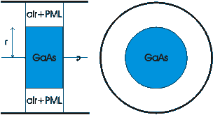
The structure defined by this script is shown in fig. 4.

A new command specifically related to circular structures is
set_circ_order(0), which tells CAMFR to look for eigenmodes with
Bessel order 0. For this Bessel order, we can have both TE and TM modes,
and in this case we choose for TE modes by setting set_polarisation(TE).
For Bessel orders other than 0, the modes are hybrid TE/TM, and any use
of set_polarisation will be ignored.
Circular waveguides are defined in pretty much the same way as slab waveguides,
except that the argument to Circ describes the structure from r=0 to
the wall, rather than from wall to wall as was the case with slabs. PML in
circular structures is set by using set_circ_PML, which adds a complex
thickness to the cladding layer.
Another new command that is introduced in this example is free_temps(),
which is called at the end of each loop iteration to free all the data
structures (eigenmodes, scattering matrices, ...) that were allocated so far.
The default mode of operation in CAMFR is to keep this data around, so that
it might be reused in future calculations. However, in this particular example,
this would only waste a lot of memory, since every iteration through the loop
creates a completely new structure with a different core width, whose results
cannot reused in subsequent calculations.
This is different from example2.py, where we did not create new
waveguides, but only varied the length of the waveguide sections.
In this case, it made sense to keep the previous calculation results around,
because eigenmode expansion can easily update the scattering matrices of a
structure if only the length of the individual waveguide sections changes.
For a more complex example dealing with Omniguide fibres, see
omniguide.py in the examples/contrib directory.
| [ < ] | [ > ] | [ << ] | [ Up ] | [ >> ] |
This document was generated by root on August, 27 2008 using texi2html 1.76.