1.3 Example 3: another stack example

In the next example, we will introduce PML boundary conditions and show how to work with files.

#!/usr/bin/env python

####################################################################
#
# Another stack example
#
####################################################################

from camfr import *

# Set constants.

set_lambda(1.5)
set_N(20)
set_polarisation(TE)

# Define materials.

GaAs = Material(3.5)
air  = Material(1.0)

# Define waveguide sections.

set_lower_PML(-0.1)
set_upper_PML(-0.1)

normal = Slab(air(2.0) + GaAs(0.5) + air(2.0))
thick  = Slab(air(1.9) + GaAs(0.7) + air(1.9))

# Calculate reflection of the fundamental mode for different 
# lengths of the central thick section.

outfile = file("tutorial3.out",'w')

for L in arange(0.000, 0.500, 0.010):    
    stack = Stack(normal(0) + thick(L) + normal(0))
    stack.calc()
    print >> outfile, L, abs(stack.R12(0,0))

outfile.close()

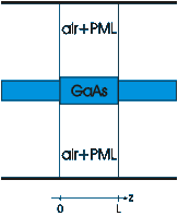
This script is very similar in structure to the previous one, and describes a waveguide with a core thickness of 0.5 micron, which widens to 0.7 um in a central section with length L (fig. 3).

set_lower_PML(-0.1) gives all the lower claddings in subsequently defined slabs an imaginary component to its thickness of -0.1j. Similarly for set_upper_PML. lower refers to the layer at x=0, which is the first term in the expression used to define the slab.

This imaginary cladding thicknesses implement the so-called perfectly matched layer (PML) boundary conditions. PML can absorb radiation travelling toward the walls, without introducing any additional parasitic reflections, regardless of wavelength, incidence angle or polarisation of the incident light. The larger the imaginary component (in absolute value) of the thickness, the stronger the absorption.

The presence of advanced boundary conditions like PML is a very powerful feature of CAMFR. Without it, the PEC walls would reflect all the incoming radiation and send it back the structure under study, where it can disturb the simulation results.

The current example also illustrates how to write output to a file, rather than to the screen:

outfile = file("myfile",'w') # 'w' indicates writing.
print >> outfile, "Hello world"
outfile.close()

This document was generated by root on August, 27 2008 using texi2html 1.76.